Chasing the Perfect Eclipse Picture 2024 by: Richard Taylor, © copyright 2024

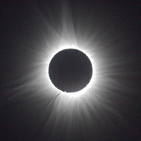
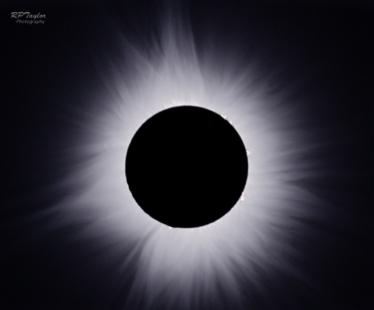
In February, 1998, I took my family on a Caribbean cruise to see a solar eclipse. Afterwards, I spent a LOT of time on the family computer trying to process my pictures into something resembling what we had seen. I was guided by an article by Gerald Pellet in the January 1998 issue of Sky and Telescope that described a technique involving subtracting images from a rotationally blurred version of the image. Eventually I described my methods on a web page that was on the RASC Ottawa Centre web site (now available at: https://web.ncf.ca/aa333/Eclipse1998/1998Eclipse.htm). I think it’s time to write an update.

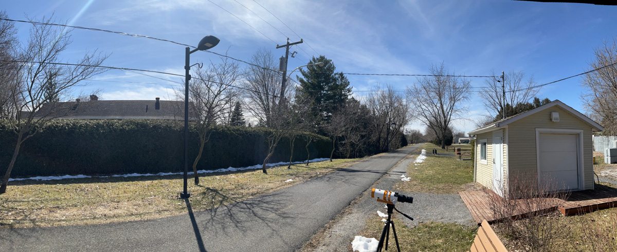
2024-04-08 was the opportunity for many Canadians and Americans to view a solar eclipse not too far from home. Recognizing that April is often a month for clouds, I was determined to keep my plans flexible until the last moment. I did ask to stay overnight from April 7 with my brother and his wife who live just inside the north edge of the line of totality, near Athens, ON. However when I saw the clouds moving in on the morning of the eclipse, I started driving down the St. Lawrence and ended up in the Eastern Townships of Quebec. The clouds kept following me, and the traffic started to get heavy. About 2pm, I got off the highway and set up my equipment in Saint-Césaire, QC, at an access point on the Route des Champs bicycle path.

This was my fourth total solar eclipse, so I knew some of the pitfalls of trying to control a lot of complicated equipment during the excitement of totality. I wanted to SEE some of the eclipse, but I also wanted a few good quality pictures with a range of exposures. My best previous picture of totality was the one from 1998, and I wanted to update the technique of rotational blur sharpening that I had used. Here is the updated technique, making use of the free image processing software GIMP. I will go through the essentials of that technique first, then add more detail about each step.

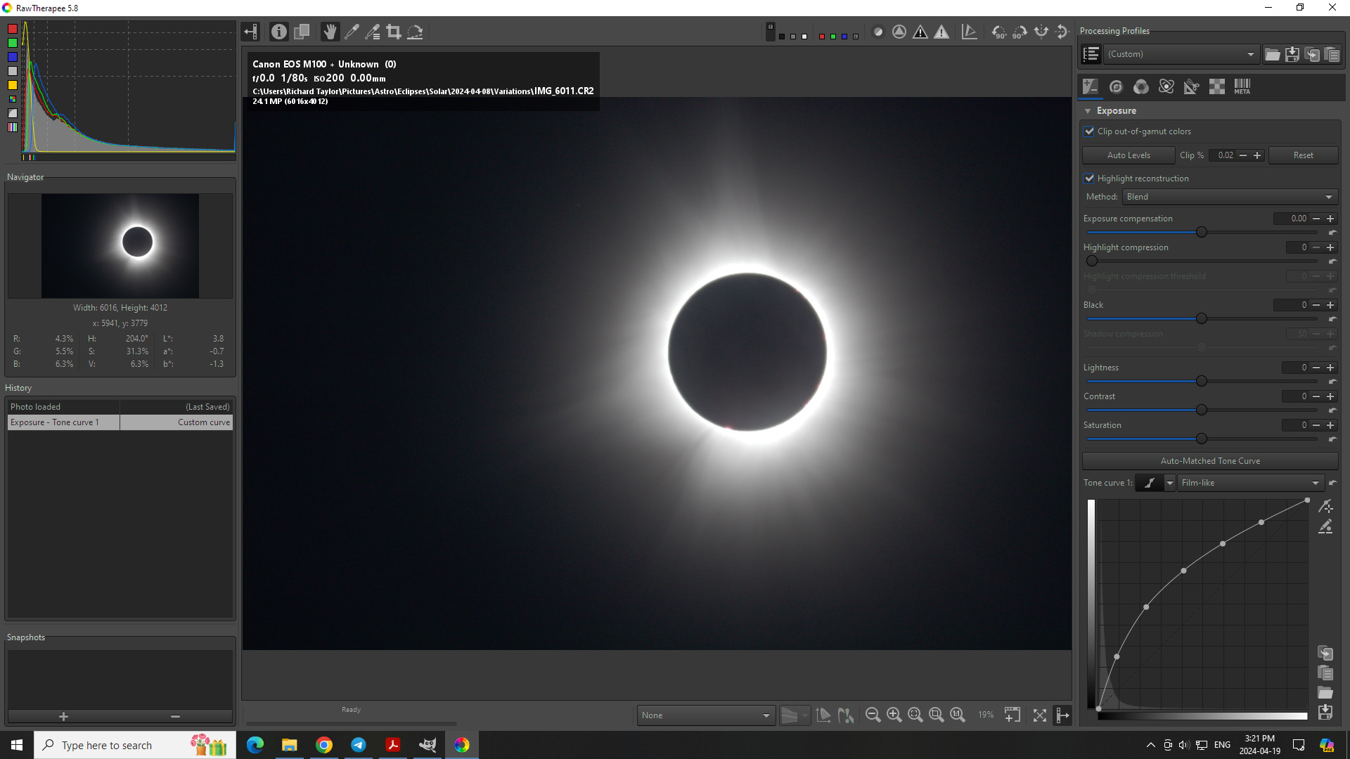
Lets start with the best quality raw image that you have. It helps to have a large number of bits per pixel as in a RAW image from a camera. The RawTherapee plugin that is associated with GIMP opens my Canon camera RAW files with the file extension ".CR2" RawTherapee also allows some initial processing of RAW files, so I used it to boost the levels with an upward curve that highlights the faint outer corona more.

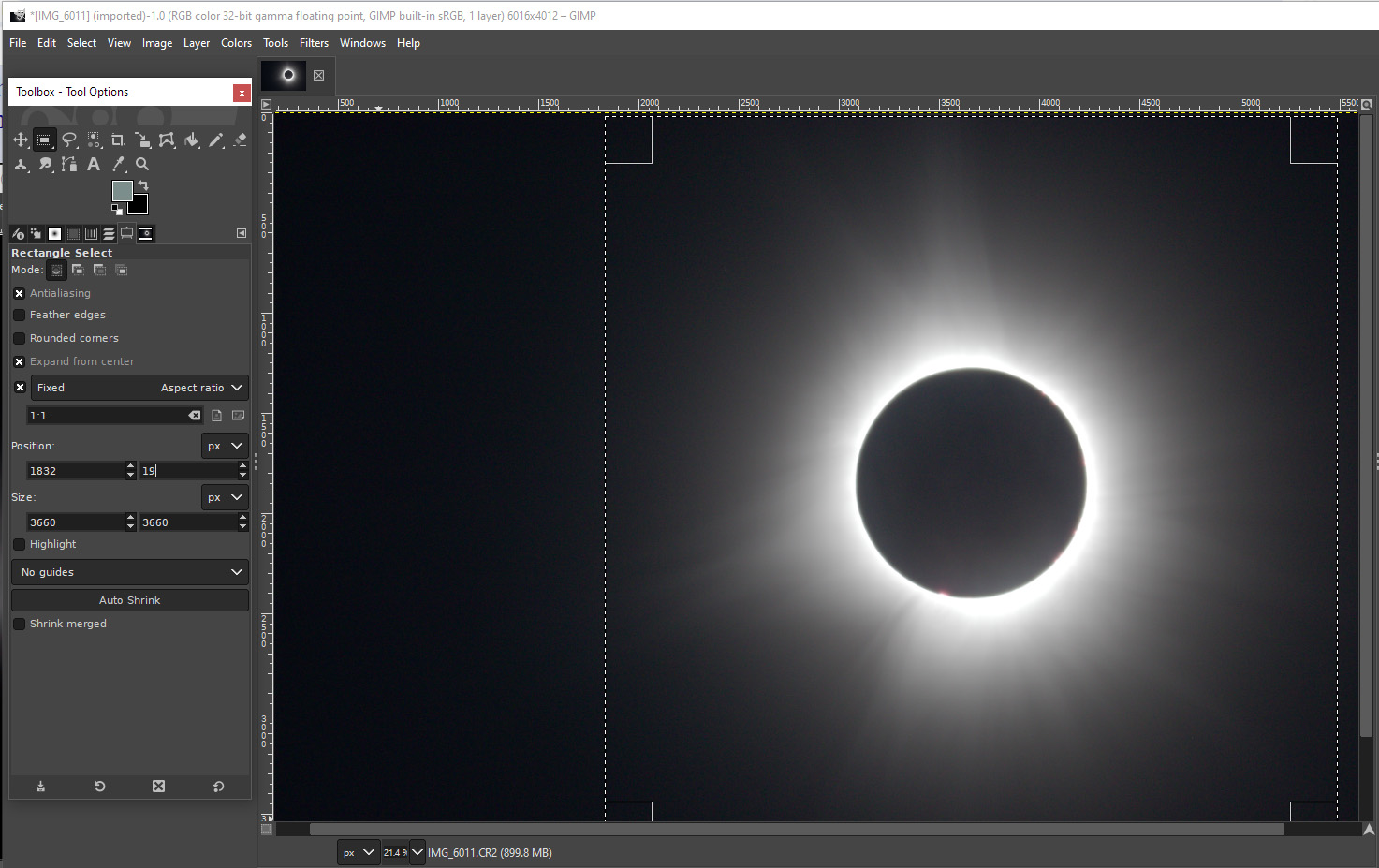
Closing RawTherapee moves the image into GIMP with the adjustments applied. In GIMP I used the cursor, the rulers at top and left and the display of the pixel position of the cursor to find tangents to the moon's edge at top, right, bottom and left. Average the x and y positions to find the coordinates of the center. Use the rectangle select tool with a fixed 1:1 ratio to select as large a square as possible centered on the center of the moon/sun.

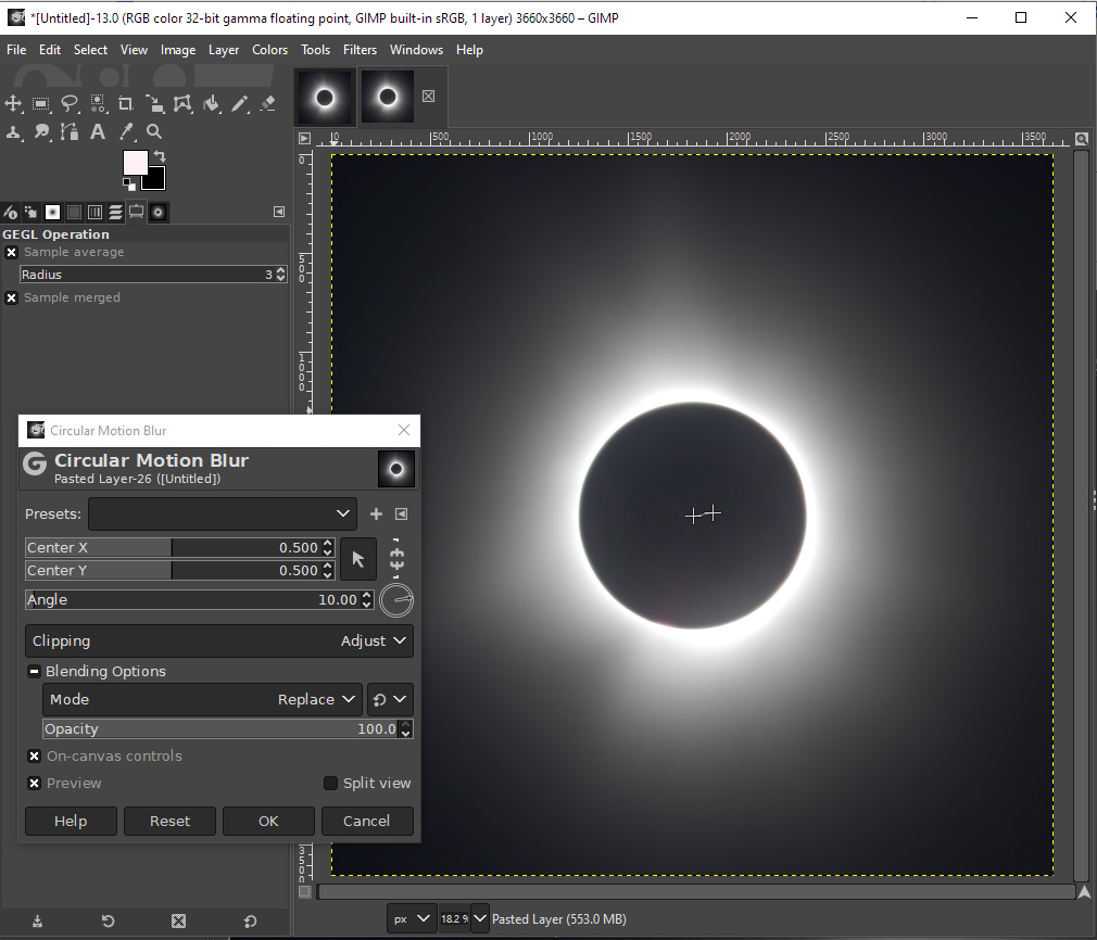
Crop the image to this selected square, then copy and paste the square image into a new image. Use Filters, blur, circular motion blur with an angle that depends on the size of the features you want to highlight. Let's use 10 degrees; that’s what I used back in 1998. Here is the rotationally blurred copy.

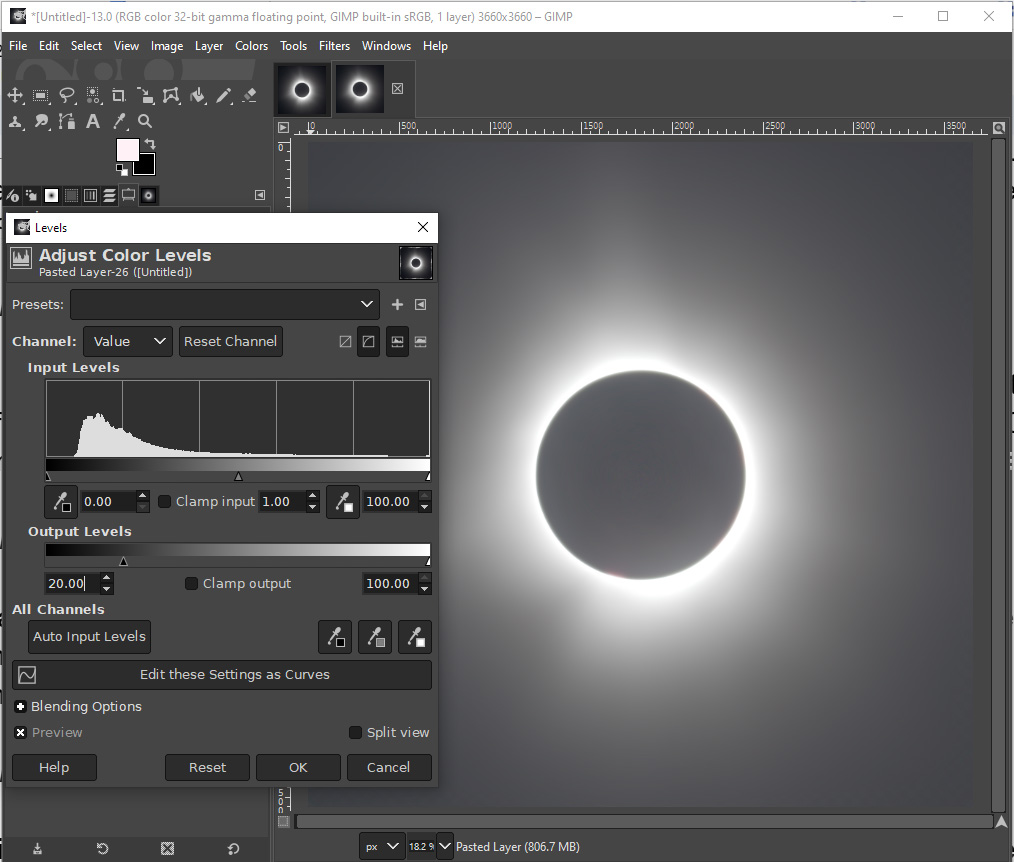
The actual difference between these two images will be the part of the original image with the most radial features. This difference is very small, and some differences will be positive and some negative, so it helps to boost the levels in the blurred copy before taking the difference. We will do this by a small amount: use Colors, levels, and adjust the output range to go from 20% to 100% as shown here:

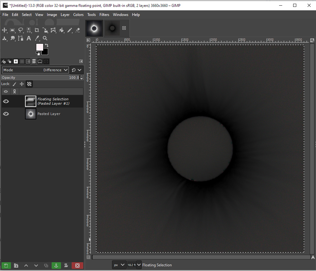
Copy and paste the unblurred image as a new layer on top of the blurred image, then select the difference operation. The result will be a negative image with a range from 0 to 20% as shown here.

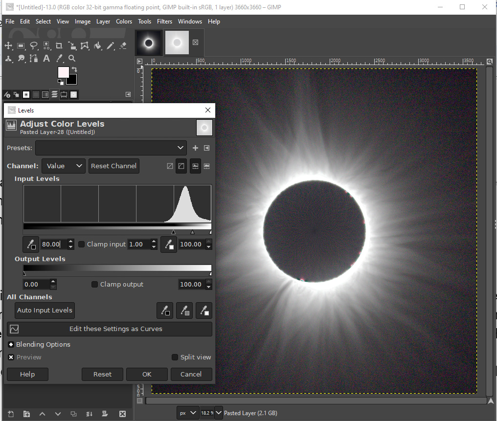
That negative image can then be flattened, Colors, invert. Then Colors, levels, set Input to the range 80% to 100%. That process brings the sharpened image back to the same brightness range as the original. Here is the sharpened image. It contains a lot more of the details of the streamers in the corona than we could see in the original.

To highlight radial features of different sizes, we can perform the same steps except change the amount of rotation of the blur. Here is a comparison of the original image with three different sharpened images. You can see that the size of the blur angle influences the size of the radial features that are highlighted.

original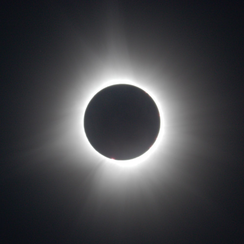

3 degree blur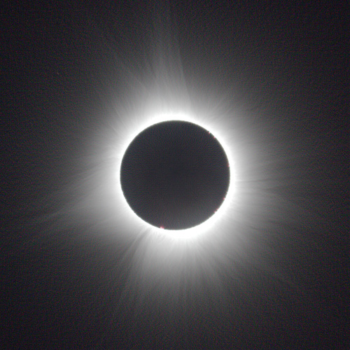

10 degree blur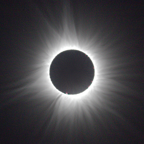

20 degree blur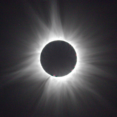

The other parameter that you can play with is the amount that you brightened the blurred image before subtracting the original image. This amount controls the range of pixel values in the difference image and thus controls how strongly the features are highlighted. Notice, however, that stronger highlighting of the features also creates stronger highlighting of the background noise. All of these images are with a 10 degree rotational blur.

5% range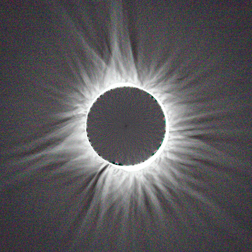

10% range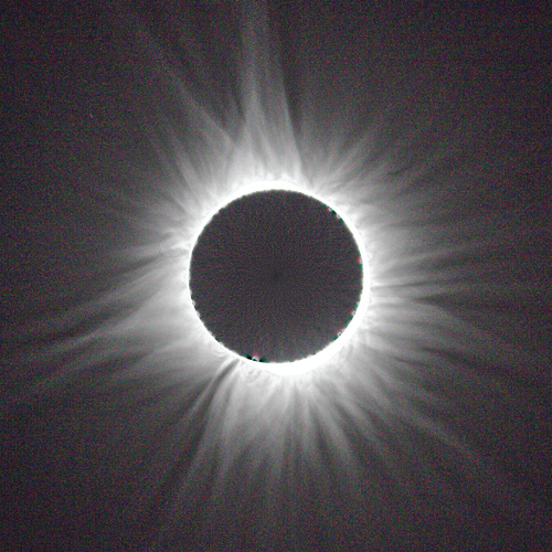

30% range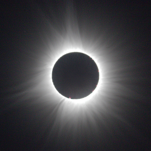

50%range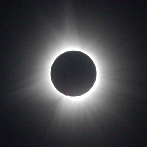

I like the amount of highlighting around the 10 percent range, but that makes for a very noisy image. It is well known that stacking multiple images reduces the noise. Stacking will also increase the “bit depth” of the image which is how many bits of information are used to encode the brightness value of each pixel. The RAW format of my Canon EOS M100 camera stores 14 bits per colour per pixel (most display screens only show 8 bits per colour per pixel.) Modern image processing software can handle 32 or even 64 bits per colour per pixel. When using larger bit depth, reducing the range of values to 10% of the original range will not introduce the graininess that we have been seeing on the examples so far.

Stacking images, especially images of different exposure lengths, is a topic I will not describe here. Basically it consists of aligning the images precisely, then averaging all the aligned images, sometimes using masking to eliminate overexposed areas.

Here is a comparison of the results. You can see that the stacking has significantly reduced the noise, as well as allowing me to show details right up to the edge of the moon. However, there are some drawbacks: I wasn’t using a tracking mount, so the image of the eclipse had a variety of positions within my field of view. That meant that the stacked image had to be cropped to the minimum size that would cover all the images - I lost some of the outer areas of the corona. Also the amazing details of the chromosphere (the prominences) are horribly distorted by the rotational blur sharpening. This last problem can be solved by pasting a single image of the chromosphere over the sharpened image and carefully matching the brightness levels.

Single image 10 degree rotation, 10% range

Stacked image, 10 degree rotation, 10% range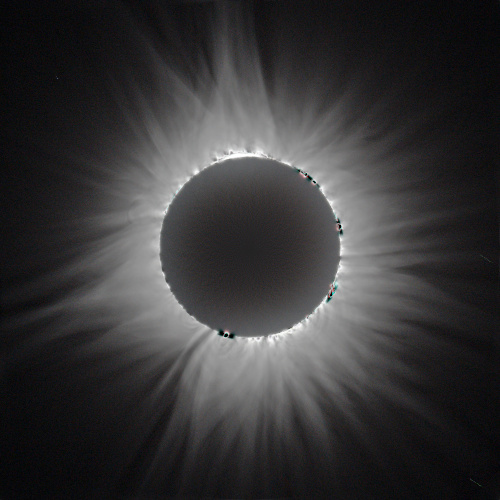

One final trick that I learned back in 1998 was a method of combining images that merges more than one level of detail. I would like to be able to show BOTH the largest and the smallest details in a single image. Well, I can do that if I combine images with a variety of amounts of rotational blur. The trick is to save the “difference” images before inverting them and simply add them up. Those dim, inverted images only use a small percentage of the possible range, so adding them just increases the range. Once added, the combined image can be inverted and the overall range adjusted as desired.

So here is my final result: stack of all the images I took during totality, rotationally sharpened with rotations of 3, 5, 8, 12 and 16 degrees, all scaled to a range of 16% and added up. Prominences retouched from my best single images.

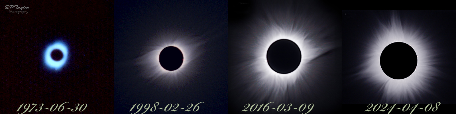
I have now gone back and reprocessed my pictures from previous eclipses (except 1973 - my skills and equipment of that time were very rudimentary and the pictures are too low resolution to be processed.) Here are the best images I have been able to produce from the four total solar eclipses that I have seen:

For more ideas on how to process eclipse pictures, especially on HDR stacking, see this Sky and Telescope article eclipse processing.