Michael Kostiuk
ABSTRACT
Determining the accurate length of the coastline is important for such coastal zone management applications as shoreline classification, erosion, biological resources, habitat assessment, and for the planning and response to natural(e.g. storm surges) and manmade disasters(e.g. oil spills).
The increasing use of spatial data and GIS (geographic information systems) by organisations and researchers is a valuable tool for coastal zone management. The effectiveness of the results obtained by using a GIS is dependent upon the quality of the data that goes into these systems. This data is known as spatial data, since each geographic feature in the database has its own geographic coordinates such as longitude and latitude. Another important aspect of spatial data is that of scale. As with a map, spatial data contains geographic information that is limited to the scale of the database. For example, a 1:100,000 scale map does not show as much detail as a 1:50,000 scale map because it displays an area that is four times smaller. The reduction of detail on maps is known as map generalisation. Map generalisation not only limits the amount of information that can be shown on a map, but it can also limit the accuracy of a map. The same is true of spatial data. Spatial data is simply map data in a digital format.
This paper will demonstrate how five different types of spatial data produce different results for shoreline length, high water area, and the number of islands in Cobscook Bay, Maine.
Determining the accurate length of the coastline is important for such coastal zone management applications as shoreline classification, monitoring erosion , mapping biological resources, habitat assessment, and for the planning and response to natural(e.g. storm surges) and manmade disasters(e.g. oil spills). The increasing use of spatial data and GIS (geographic information systems) by organisations and researchers is a valuable tool to help solve the planning and management issues in the coastal zone (Canessa & Keller, 1993). Geographic information systems can be defined as computer based systems that process georeferenced data through various means such as data encoding, data management, geographic analysis and output (Aronoff, 1991). Georeferenced spatial data is map data in a digital form which means that each of the earth's features that are stored as spatial data has a unique geographic reference such as latitude and longitude. There are many different geographic information systems in use today and they tend to differ in certain aspects such as: "how they link geographic locations with information about those locations, the accuracy with which they specify geographic locations, the level of analysis they perform, and the way they present information as graphic drawings" (GeoInformation International, 1997 p 1-4) .
A definition of the coastal zone is somewhat ambiguous since it can include an area that is as small as a buffer zone that ranges several kilometres from the shore line, or it can extend inland to cover entire inland watersheds and/or extend into the sea to include the continental shelf and a country's 200 nautical mile Exclusive Economic Zone (Hinrichsen, 1998; OECD, 1993). What constitutes the coastal zone will not be covered in this article as it would warrant its own article to say the least, but instead this paper will focus on the accurate measurement of the coastline by a Geographic Information System through the use of various spatial data. For this article, an area of coastline known as Cobscook Bay, Maine will be used as case study to show how different types of spatial data can produce quite different results when used in a geographic information system. Along with the measurements of the shoreline, several other elements of the coastline will also be measure such as the number of islands in the bay, the area of the islands, the length of the shore line of the mainland and of the islands, and the water area of the bay itself.
The coastline is the geographic centre of the coastal zone and it is also the location from where the coastal zone is defined. The location of the coastline depends on what datum is used for the sea level, and whether the high tide, or low tide level is to be used as the point of reference. In the case of Cobscook Bay, since it is so close to the Bay of Fundy, there is a large difference between the low and tide levels. The mean tidal range of Cobscook bay is 5.7 metres or approximately 18.7 feet, and this is the highest tide that can be observed in the United States of America (Brooks, D.A, Baca, M. W., & Lo, Y.-T, 1999). Consequently, such a large tidal range as this produces two very different coastlines at the high and low range of the tide cycle. In this paper, the measurement of the coastline will be done at the mean high water tide levels as shown on the USGS 1:24,000 scale quadrangle maps, and the Mean Sea Level (MSL) that is used by the 1993 version of the Digital Chart of the World (Maine, Office of GIS, 2000 ).
There are many parameters to consider when using a geographic information system to measure selected features on the earth's surface. As has already been mentioned, there is the problem of which vertical datum to use to define the coastline. Some of the factors that also must be considered are:
- The type of spatial data.
- The scale and resolution of the spatial data.
- The type of map projection.
- Map generalization.
- The measuring unit.
- Horizontal and vertical datum for the geographic coordinates
And
- Metadata.
While a thorough explanation of the complexities of these important factors is well beyond the scope of this paper, many of these contributing conditions will be discussed throughout this article and are briefly summarized below:.
Analog Maps, Digital Spatial Data, and GIS.
The usefulness of a paper map(analog data) is limited to its scale, however once a map and its geographic features are stored as digital data it can then be manipulated in a geographic information system. Once a map is in a digital format it can be modified and loaded into a wide variety of computerized drafting, automated mapping and geographic information systems. According to Jenson (1996), there are basically four types of spatial data: 1) Traditional Cartesian vector(Sometimes know as spaghetti), 2)Topological vector, 3)Raster, and 4)QuadTree Raster .
The traditional Cartesian vector system stores geographic locations as points, lines and polygons. A point is recorded with an "x" and "y" coordinate. Lines are recorded as a series of "x" and "y" coordinates, and polygons are recorded as series of "x" and "y" coordinates forming a closed loop. The "x" and "y" coordinates are known as vertices. One of the drawbacks of this method is the possibility of over digitizing features when geographic entities share a common border. The result of this type of duplication can result in the creation of geometric errors sometimes knows as slivers.
Topological vector systems use a node and arc system to store spatial data. Like the cartesian systems, geographic locations are stored as points, lines and polygons.
A line is an ordered set of points that describe the position and shape of a linear element on the map and each line starts at a node, and ends at a node (USGS, 1997 p. 16). The beginning and the end of geographic features are designated with a node, and the nodes are linked to other nodes with arcs. If proper procedures are followed, this system does not allow for the duplication of geographical features as is the case with Cartesian based vector systems, and consequently fewer geometric errors are produced.
Raster data stores geographic information as a cell within a grid and each cell within the grid is identified by a row and column. Each cell is also identified by a geographic location and it can also be linked to a particular geographic feature such as a body of water or a type of land cover. These cells are sometimes referred to a pixels when they are display on a computer screen. Cell size can range from 1 metre (1 x 1 m) resolution for USGS Digital Orthophoto Quadrangle(USGS, 2000), to 30 metre (30 x 30 m) resolution for Landsat 5 Thematic Mapper images to 315 kilometre (315 x 315 KM) resolution for Nasa TOPEX/POSEIDON Nonimaging radar(Jensen, 1996).
Quadtree raster data is similar to traditional raster data except that larger cells are used to represent areas that have the same type of geographic feature and smaller cells are used to encode areas of high spatial heterogeneity (Laurini & Thompson, 1992). Quadtree raster systems can store data more efficiently than a traditional raster system if the "mapped" area contains zones of homogeneous land cover. Raster data typically stores geographic data more efficiently than vector data, but vector data tends to be of a greater geometric accuracy.
There is no single accepted standard for storing geographic data, and consequently many organizations and GIS companies have developed their own methods for storing spatial data. Not surprisingly, the wide variety of different styles of spatial data has created numerous problems for organisations and people that want to use spatial data in their geographic information systems. To use spatial data from a variety of sources in a GIS , a conversion utility must be used in order to convert the data into a form that can be used by the GIS. Some of these utility programs are quite straightforward to use, but unfortunately others can be quite complicated and tedious to use. When the GIS professional uses certain proprietary programs to convert GIS data from one format to another format, there can be potential problems if the computer code that performs the conversion process, is in hidden within the utility program. In these situations the GIS user must trust that the organization that produced the utility used the correct and best set of mathematical algorithms to do the conversion.
Scale
A map scale is a representation of the ratio between a measurement of distance on a map to the same distance in the real world. For example, a map feature that is 2 centimetres long on a 1:50,000 scale map represents an object that is 100,000 centimetres or 1000 metres(1 Kilometre) in the real world. The larger the scale factor becomes, the smaller the map scale becomes, and the opposite is true as well. As a general rule, as the scale of the map increases, there will also be an increase in the accuracy of the map, and there will also be an increase of the amount of geographic features that can be displayed on the map. When using spatial data for mapping and measuring purposes, the largest scale maps and spatial data that cover a selected study area should be obtained for use in a geographic information system. If spatial data that was created on small scale is used to produce a map at a larger scale then this violates how data should be used in a GIS. Goodchild and Gopal(1989) wrote about the importance of applying the correct accuracy to the output of a GIS so that it does not exceed the accuracy of the spatial data was used to create the new GIS file. The following quote was the from preface of book on the Accuracy of Spatial Databases:
GIS designers typically carry the maximum precision through GIS operations, and print the results to a precision which far exceeds the level justified by the accuracy of the data. In part this may be due to a lack of appropriate methods for describing and tracking accuracy, and in part to a reluctance to throw away digits, however meaningless they may be (pp. xii-xiii).
Spatial Resolution of Data
The degree of resolution of spatial data is important for the user of geographic information systems. The spatial resolution of GIS data is also a function of generalization since small scale maps do not usually contain as much geographic detail as larger scale maps, and as a result, the data is most often recorded and stored with less spatial precision. For vector data, spatial accuracy is a function of how many nodes and vertices are used to record geographic features at a particular map scale. The closer the vertices are to each other, then the degree of resolution of the spatial data also increases. The farther apart the vertices are from each other, then the reliability of the spatial data to represent geographic features in their true shape and size will diminish accordingly. This is especially true for rivers and coastlines where their shapes and orientation can constantly change across the earth's surface. A coarse spatial resolution has the effect of straightening out a meandering feature, which gives it a smoother appearance and as a consequence, its recorded length becomes shorter as well. Robinson et al (1978), describes resolution in vector digitizing by "changes in the size of the minimum increments between adjacent data points in the x and y directions. Greater resolution is achieved by specifying finer increments"(p. 417). If a coarse spatial resolution is combined with a small scale map, the spatial data cannot be relied upon to accurately record or display geographic features. This problem will be demonstrated in the latter half of this article.
Map generalisation
Unless a map is compiled at a scale that is the same as reality, or at a 1:1 ratio, the cartographer is forced by necessity to limit the amount of geographic information that can be shown on a map. As a map scale gets smaller, less and less information can be shown on the map due to the limitations of available space and the problems of representing a feature at its true size. On smaller scale maps, geographic features such as roads, railways, rivers, shorelines of lakes, coastlines of the mainland and islands are simplified (or they are removed) to make the map easier to read and understand. As the map scale becomes ever smaller, the width of the line that is drawn on the map to represent a geographic feature becomes a major determining factor as to what type of geographic information can be successfully depicted. For example, a line that is printed at a width of 0.8mm on a 1,1:000,000 scale map to represent a road that is 20 metres wide actually takes up 800 metres of space on the map. It is necessary to exaggerate the dimensions of many geographic features on small scale maps so that they can be clearly seen by the map user. In the case of the above example, if the road was drawn to its true scale, the line would have a width of 0.02mm which is too far too small for most people to clearly see. On medium and small scale maps, symbols are also used to represent geographic features that would normally be too small to recognize if they were printed at their true size. On all but the largest scale maps such as 1:2,500 maps (that are also known as plans), many geographic features have to be exaggerated in size in order for them to be clearly seen (Robinson et all, 1978) . Many large scale maps plans are produced using such strict and precise survey methods that their accuracy is so good that the map data can "have the validity of legal documents and are the basis for boundary determination, tax assessments, transfers of ownership, and other functions that require great precision" (Robinson et all, 1978, pp. 7-8). Map generalisation may be accomplished manually by a cartographer or it can be done through a computerized process.
Projections
The earth is a sphere that is slightly flattened in the polar regions, and to draw a large portion of the earth's surface onto a flat piece of paper has always been a problem and a challenge for map makers. There are over 250 different map projections and each one has its own particular strengths and specific uses. Some projections are better for the accurate representation of certain regions of the world, while other projections are designed for a specific purpose such as showing true directions for navigation (but not true distance) such as with the famous Mercator projection that many people remember from their school days. All map projections will distort the earth's sphere to a certain degree especially regarding the representation of angles, area, distances and direction. (Robinson, Sale, Morrison, Muehrcke, 1984). The choice of a particular map projection depends on which portion of the world is to be displayed and measured.
The measuring unit
Different maps can be based on different types of map measuring units. Spatial data can be stored in various types of units such as decimal degrees, metres, or feet. It is important to know what unit the spatial data uses so that the correct scale can be applied to the map. If an incorrect measuring unit is applied to spatial data that is loaded into a GIS, then a false map scale will be the result. If the map scale is incorrect, then all of measurements using a GIS will be wrong. Spatial data will often be stored using decimal degrees as the map unit, and that makes it easy to project the data into a variety of map projections. Certain types of spatial data such as GIS data from some local governments in the United States are stored as feet using the State Plane Coordinate system( ArcView GIS 3.2). Other map projections such as the UTM(Universal Transverse Mercator), can use metres as the measuring unit. When GIS data is obtained for use in a GIS, it is very important to know what the map units are, and this information is usually contained in the information file that comes with the spatial data. The information file is normally named "Metadata".
Horizontal and vertical datums
Map datums refer to the various locations from where geographic measurements are referenced, and this is one of the parameters in which individual maps are identified. Many North American maps have been, or will soon be converted to a new horizontal map datum known as NAD83. This new datum is replacing the NAD27 which was based on the Clark spheroid of 1866 that was used to represent the shape of the planet.
The centre of this datum is located on a section of the Meades Ranch in Kansas and other NAD27 control points across North America were referenced to this location. As more efficient and reliable survey methods were developed over the years utilising advances in the areas of computer assisted surveying, to satellite positioning systems, it became apparent that there were substantial errors in the NAD27 datum.
The newer North American datum known as NAD83, is an improvement over the older NAD27, and it is based on the GRS80(Geodetic Reference System) spheroid. The GRS80 spheroid in turn was developed from the World Geodetic System ellipsoid of 1984 spheroid. WGS84 is the name of the datum that is based on this spheroid. Global Positioning Systems use, and are based on WGS84 (Owens, 2000). The WGS84 and NAD83 spheroids both use the centre of the earth as the location of the datum. The NAD83 and WGS84 datums are essential the same datums, except that NAD83 is designated for civilian, and North American use, while the WGS84 datum is the term used for military users( USGS, 1998).The use of these newer datums has meant that maps that are based on the NAD27 datum can be shifted as much as 150 metres in the horizontal direction as compared with NAD83/WGS84 based maps that cover the same area(ArcView GIS 3.2). Conversion programs are available that can update the horizontal positions of NAD27 maps to match the horizontal positions of NAD83/WGS84 maps.
Vertical datums
Along with horizontal datums, maps are also referenced to vertical datums. According to Wolf and Brinker (1989) a datum is "any level surface to which elevations are referred (for example, mean sea level). Also called datum plane, though not actually a plane" (p. 108). In the United States of America, the vertical datum known as NGVD29(National Geodetic Vertical Datum) was established by the U.S. Coast and Geodetic Survey's 1929 General Adjustment(USGS, 1998). In Canada, the vertical datum are expressed in reference to the Mean Sea Level (Canadian Vertical Geodetic Datum) (Canada, Geomatics Canada, 1996).
Another type of datum is the MSL(Mean Sea Level), which is based on the average height of the sea's surface for the complete tidal ranges over a 19 year period. Other vertical datums are based on the various Tidal Datums which are used in coastal zones to establish property boundaries of lands bordering waters that are subjected to tides (Wolfe & Brinker, 1989).
Metadata
GIS data normally comes with a file of information that describes the content of the data sets. This particular GIS information file is commonly known as Metadata, and it describes the basic features of the GIS data. For the Metadata to be useful, it should list the map title, spatial area covered, the map projection, the horizontal and vertical datums, the map units, the version number of the map, the date of the map, mapping specifications, and accuracy limits. The United States Geological Survey document Standards for the Preparation of Digital Geospatial Metadata lists the following rules for metadata:
"Identification information provides basic information about the data
set, including the title, geographic area covered, currentness, and
rules for using the data. Required elements of metadata are those
necessary for identification of the data set and include citation,
description, time period of content, status, spatial domain,
keywords, access constraints, and use constraints. The
identification information is a mandatory element of the data set
metadata" (USGS, 1997, p. 2-1).
Sometimes the spatial data contains no Metadata, and this can cause problems when you need to know important map features such as datums and map units. In other cases, the metadata may be available on an organization's web site, or it may be available as a printed set of mapping specifications that is mentioned in the metadata. Sometimes the Metadata can be located through a combination of all three of the methods that have just been described.
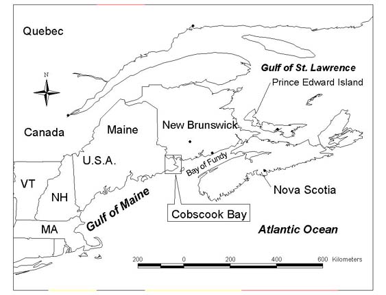
Cobscook Bay is located in the southeast corner of the American state of Maine. The bay consists of many coves, numerous smaller bays, and harbours. There are also many islands and rock ledges within Cobscook Bay. The two largest communities that border the bay are Eastport and Lubec, both of which have populations of approximately 2000 people. Eastport is the eastern most city in the United States, while Lubec is the eastern most town. Eastport was once the home to a thriving sardine canning industry at the turn of the 19th and 20th centuries when it could once boast having as many as 18 sardine canneries (Holt, 1999). Between the two world wars, the number of canneries were reduced from 18 to 5 through mergers and the elimination of unprofitable and inefficient operations. Eastport had a population of 5,311 in 1900, but the city experienced negative growth in the early decades of the 20th century, and the crash of the sardine industry in the 1950s further reduced both the number of sardine canneries, and the population of Eastport (Holt, 1999). The last operating sardine cannery closed in Eastport in 1983 while there is still one cannery operating out of Lubec. Today, the aquaculture industry has replaced many of the traditional fisheries in the area and Cobscook Bay is an important location since its sheltered bays are ideal for the location of the fishpens. Cobscook Bay was also once an important location for the harvesting of various types of shellfish such as the many clam, and scallop species that are traditional to the area. Unfortunately, many of the clam beds are sometimes closed due to Faecal Coliform Bacteria pollution, and at other times, the shellfish cannot be sold on the commercial market if they have become contaminated with one of the various diseases such as PSP(Paralytic Shellfish Poison, or sometimes referred to as Red Tide), or ASP(Amnesic Shellfish poisoning). There is also a concern that the high concentration of aquaculture fishpens has contributed to the algae growth (such as enteromorpha that grows on the tidal flats) in the local area by adding excess nutrients into the water column of the Cobscook Bay and the surrounding waters. Studies of tidal currents in Cobscook Bay by Brooks et al.(1999) have reported that "the tidal-mean flushing times for neutral surface particles in Cobscook Bay vary from less than one day in the eastern arm near Moose Island to greater than one week in the extremities of the inner arms of the bay" (p. 663). Currently, most of the aquaculture sites are located in the centre or eastern part of the bay where the tidal cycle is strong enough to "carry away the waste products, and to also bring in new supplies of dissolved oxygen"
( Brooks et al, 1999 p. 664).
- macro(1:1,000,000 - 1:2,000,000 scale) level for a large area coverage.
- meso(1:50,000 - 1:250,000 scale) for semi-detailed depiction of features.
- micro(1:5,000 - 1:10,000) level for a high level of accuracy and detail.
Commenting on the above categories, Canessa and Keller (1996) reported that, "data for a coastal zone GIS inventory should be collected and explicitly tagged to belong to one of the three planning levels. If collected at one level, they should not be accessed at a larger scale" (p. 106). These three categories of scales for map usage are not continuous, and there are is no mention where other map scales such as 1:25,000 maps are to be allocated.
For the GIS analysis of Cobscook Bay, I am concerned with the accurate measurement of the coastline, and therefore, it is important to determine a minimum acceptable scale that will be useful for that purpose. In 1991, Peter Wainright along with the Canada Department of Fisheries and Oceans published a report titled Fisheries Habitat GIS Strategy and it contained recommendations for minimum scales for use in measuring shorelines and watersheds.
The following is quote is from that report:
"The map scale recommended as a "standard" must be appropriate to the most demanding, priority use. That is, other scales could be used for special purposes, but should not be advocated as a broadly applicable standard. Water bodies must posses enough resolution to describe reaches. Coastline must have enough detail to describe shoreline units. Reaches may be as small as a 50 m section of a stream. Shoreline units are normally larger, but may be as small as a100 m section of shoreline. On a 1:50,000 scale map a 50 m section of stream would be I mm in length. Therefore, mapping at 1:50,000 scale is not suitable for habitat information needs " (p. 14).
This report describes that a minimum acceptable scale to portray the coastline should be at a 1:40,000 scales and larger, and that the minimum scale for watershed mapping should be at the 1:20,000 scale (Wainright, 1991). For the GIS analysis of Cobscook Bay, this 1:40,000 scale recommendation will be used as the desired minimum acceptable scale to measure the coastline of Cobscook Bay and then compare it to other scales to see how close or how far that they are able to accurate represent the size and dimensions of the bay. It should be noted that the minimum scale of 1:40,000 falls in between the micro and meso map categories that was described by Cedero.
Coastline Data
Cobscook Bay was analysed using ESRI's ArcView 3.2 geographic information system running on a 450 MHZ Pentium III based microcomputer. The spatial data for the analysis was obtained from the following sources:
1) Maine Office of GIS internet site at http://apollo.ogis.state.me.us
2) The United States Geological Service Coastline Extractor at USGS Coastline Extractor
3) Pennsylvania State University's Maps Library site at DCW from Penn. U.
All of the spatial data were available as a free download from these sites and their original copyrights are still in effect.
The spatial data from the Maine Office of GIS were downloaded as zipped ArcInfo (A gIS made by ESRI) format files at scales of 1:24,000 and 1:100,000. The Maine Office of GIS organises their spatial data according to map layer features and to various types of coverage areas. Each type of spatial data is identified by a geographic name, an attribute such as road or shoreline, and a map scale. The data were digitized from the Mean High Water (MHW) line as shown on USGS 1:24,000 scale quadrangle maps. The accuracy limits for the 1:24,000 scale data is that " not more than 10 percent of the points tested shall be in error by more than 1/30 inch, measured on the publication scale" for horizontal accuracy(ground scale), and "that not more than 10 percent of the elevations tested shall be in error more than one-half the contour interval for vertical accuracy" (USGS, Part 1, 1997, p.1.D-2) . The accuracy limits for the 1:100,000 scale data are that at least 90 percent of points tested are within 0.02 inch of the true position (ground scale) for horizontal accuracy and that at least 90 percent of well-defined points
tested should be within one-half contour interval of the correct value for vertical accuracy (USGS, Part 3, 1997, pp. 3-12,3-13). The projection is UTM Zone 19, that uses the NAD83 horizontal Datum, and the units are in Metres.
The spatial data that was obtained from the The United States Geological Service Coastline Extractor were zipped Arc Ungenerate format files that can be used by the ESRI ArcInfo GIS. The data was in the form ofNOAA/NOS Medium Resolution Digital Vector Shoreline at a scale of 1:70,000. This data was a portion of a larger data set that covers the entire United States of America. This data was digitized from NOAA nautical charts. The other set was a portion of the World Vector Shoreline which is at the 1:250,000 scale. This data can be used for world wide coverage. Both of these data sets only contain line information, and since no polygons are included with these data sets, only the lengths of features can be easily measured.
For the 1:70,00 data, the horizontal datum is NAD83, and the vertical datum is (NAVD29) which is based on the mean high or mean higher high shoreline position on published nautical charts. The spatial resolution of the data set is set to a minimum adjacent vertex spacing of five metres ground distance. The source of the spatial data are from the master copy of the National Ocean Service's coast charts, and they are supposed to meet or exceed National Map Accuracy Standards (Rohmann, 2000).
The 1:250,000 data uses the WGS84 horizontal datum and the horizontal accuracy requires that 90% of all significant shoreline features are to be located within 500 metres (or 2.0mm at 1:250,000 map scale) circular error of their true geographic positions. The vertical datum is based on the mean high water mark designated MHW.
The original source of this data is US Defence Mapping Agency now known as the National Imagery and Mapping Agency or NIMA (Soluri & Woodson, 1990).
The spatial data from the Pennsylvania State University's Maps Library site was also in the form of zipped ArcInfo format files, but it was downloaded as one single file that covered the entire state of Maine. This spatial data was a portion of the Dataset from the larger spatial dataset that is known as the Digital Chart of the World or DCW. The scale of the DCW spatial data is 1:1,000,000. Elevation datum is Mean Sea Level (MSL). The horizontal datum is WGS84, and the horizontal accuracy, "at a 90 percent confidence level for circular error, ranges from 1,600 feet to 7,300 feet. The vertical accuracy, at a 90 percent confidence level for linear error, ranges from 160 feet to 2,100 feet" (Environmental Systems Research Institute, Inc. 1993, p. 2-13).
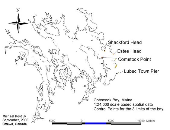
The boundary and extent of Cobscook Bay is also not agreed upon by various people and organizations who are familiar with the area and there are at least three definitions of its geographic limits. All of the three definitions of Cobscook Bay include all of the inner bays and extend to the following limits:
- Comstock Point to Shackford Head.
- Comstock Point to Estes Head.
- Estes Head to the town pier in Lubec, Maine.
Therefore, to make this analysis of the Bay as thorough as possible all three boundaries of Cobscook Bay were measured using the spatial data that was obtained for this study. The results of this analysis are listed in three tables in the conclusion of this paper.
The same basic methodology was used on each set of spatial data to obtain the various measurements of the lengths of shorelines and the areas of the three different Cobscook Bay limits. The first step was to convert the spatial data into an ArcView shapefile, and then to load the shapefile into the ArcView GIS. The next step is to change the projection to a UTM(Universal Transverse Mercator) projection. The use of the UTM projection was selected so that metres could be used as the measuring unit, and to have consistency between the various types of GIS data. The UTM zone was set to zone 19 which covers the area of Maine, and the map's horizontal datum was set to NAD83.
The UTM projection is a similar to the Mercator projection except that the cylinder is longitudinal along a meridian(Longitude line) instead of the Equator. The result is a conformal projection that is divided into 60 zones of 6 degrees width. The UTM projection's properties are to be able to represent an accurate depiction of smaller shapes, and at the same time, with a minimal distortion of larger shapes within the zone. Local angles are also true within each zone. These zones are numbered from 1 to 60 and this provides 360 degree coverage of the earth from 84 degrees North to 80 degrees South. Each zone also has its own central meridian and it covers an area of 3 degrees east and west of the central meridian. Horizontal lines are designated using metres that are measured from the equator. North of the equator, the North origin or "northing"is given a false value of 0 degrees and South of the equator the origin of the northing is given a false value of 10,000,000. Vertical lines are measured from a "false" point 500,000 metres to the west of each zone. The central meridian has a value of 500,000 metres, and all points to the west of the central meridian decrease in value to the origin at 0 while all points to the East of the central meridian increase in value to the zone's limit at 1,000,000. A grid square grid is placed over this projection, and positions on the map are located using the UTM grid system of Easting and Northings along with the zone number. The UTM projection is used by civilian mapping organizations such as the United States Geological Service, and Natural Resources Canada. The UTM projection is also use by many military mapping establishments such as the NATO member countries. The military users have also their own unique reference system for reference on UTM maps called the Military Grid System.
Next, the data was matched to the same geographic limits of Cobscook Bay. This was accomplished by a technique known as the clip theme operation or sometimes it is known as the "cookie cutter approach". A template that matches the limits of Cobscook Bay is created, and then saved as a polygon shapefile. This template is used to cut away the excess spatial data from the selected spatial data set, and the output is saved as a new ArcView shapefile. This technique works for both line and polygon data. Point data can also be selected using a theme on theme selection process, or by using the geoprocessing wizard that comes with ArcView 3.2. An ArcView programming script called "calcapl.ave" is run on the new spatial data for the purpose of recalculating the lengths, areas and perimeters of geographic features. The results of these operations are then saved in their associated database tables. If these new measurements are not made, then the dimensions of the geographic features will be based on their previous extents. The end result is a new set of spatial data that contains tables and spatial coordinates that match the specified limits of Cobscook Bay. This operation is run three times so that the three limits of Cobscook Bay can be measured. Control points that represented the three limits of Cobscook Bay were established on the 1:24,000 scale GIS files of Cobscook Bay(The largest and most accurate set of spatial data). Their UTM coordinates were obtained by running a program script, and these control points were then copied to the other four scale-based sets of GIS files. In this way, the templates that were used to create the new data sets for each scale of GIS data used the same control point(based on UTM coordinates) on each map.
The new sets of spatial data can be used to find the lengths of shorelines and areas of water bodies and islands of Cobscook Bay, Maine. This geographic information can be obtained by several methods such as using a query function in the corresponding map tables, or by selecting the features on the screen and going back to the tables to see the results.
Metres
1:24,000
1:70,000
1:100,000
1:250,000
1:1,000,000 Length of
Mainland
Shoreline
357,856.5
Metres
315,816.5
Metres
299,445.9
Metres
192,493.9
Metres
168,850.6
Metres Length of
Island
shorelines
57,482.0
Metres
51,674.5
Metres
31,786.8
Metres
20,884.8
Metres
0.0
Number of
Islands
169
87
29
10
0 Area of
Cobscook Bay
89,946,702.67
SQ. Metres
N/A
90,197,323.7
SQ. Metres.
N/A
94,019,162.5
SQ. Metres Area of
Islands in
Cobscook Bay
2,404,855.7
SQ Metres
N/A
1,962,162.4
SQ Metres
N/A
0 SQ Metres
| 1:24,000 | 1:70,000 | 1:100,000 | 1:250,000 | 1:1,000,000 | |
| Length of Mainland Shoreline | 363,499.8 Metres | 321,249.2 Metres | 304,562.3 Metres | 198,361.3 Metres | 171,969.8 Metres |
| Length of Island Shorelines | 57593.0 Metres | 51,674.5 Metres | 31,786.1 Metres | 20,884.8 Metres | 0.0
Metres |
| Number of Islands | 171 | 87 | 29 | 10 | 0 |
| Area of Cobscook Bay | 92,070,024.6 SQ. Metres | N/A | 92,297,119.9 SQ. Metres | N/A | 95,991,319.6 SQ. Metres |
| Area of Islands in Cobscook Bay | 2,405,224.3 SQ.Metres | N/A | 1962162.4 SQ.Metres | N/A | 0.0
SQ. Metres |
Dimensions of Cobscook Bay, Maine, USA.
Estes Head to Lubec Town Pier
| 1:24,000 | 1:70,000 | 1:100,000 | 1:250,000 | 1:1,000,000 | |
| Length of Mainland Shoreline | 380,900.4 Metres | 335,820.5 Metres | 317,125.4 Metres | 220,612.8 Metres | 180,019. Metres |
| Length of Island Shorelines | 60,860.7 Metres | 55,709.6 Metres | 35,737.4 Metres | 25,917.6 Metres | 1,223.8 Metres |
| Number of Islands | 186 | 95 | 33 | 13 | 1 |
| Area of Cobscook Bay | 100,536,850.3 SQ. Metres | N/A | 100,534,727.2 SQ. Metres | N/A | 105,004,515.8 SQ. Metres |
| Area of Islands in Cobscook Bay | 2,639,025.3 SQ. Metres. | N/A | 2,181,156.5 SQ. Metres | N/A | 201,450.4
SQ. Metres |
Several things are quite evident from the above tables. As the scale of the maps and spatial data decreases, so does the length of the shorelines of the mainland and those of the islands also decrease in length. This is due to the decrease in spatial resolution and the amount of generalization of geographic detail that occurs as the map scale becomes ever smaller. On the other hand, the water area of Cobscook bay tends to increase in size as the scale gets smaller. This is due to the elimination of smaller geographic features such as islands which by default, will create more open water area. The generalization of geographic features can also create more open areas or, it can sometimes reduce the amount of open water area if the land area is generalized over a water area. I was also able to obtain spatial data at a scale of 1;24,000 which is above the minimum requirements that was described the Wainwright/DFO report of 1991. As can be seen from the tables, the size of a geographic feature that is measured using spatial data in a GIS becomes more precise as the scale becomes larger and less precise when the scale becomes smaller. Small scale maps are fine for the depiction of geographic information that covers a large area. When accurate measurements of geographic features are required, then a minimum acceptable scale must be established so that a higher degree of precision can be obtained. The scale of the spatial data should also be included as part of the GIS analysis for reference purposes.
ArcView GIS 3.2. Computer Software. ESRI(Environmental Systems Research Institute,
Inc.) ( 1999).
Aronoff S. (1991). Geographic Information Systems: A Management Perspective
( p. 294) Ottawa: WDL Pub.
Brooks, D.A., Baca, M. W., & Lo, Y.-T. (1999). Tidal Circulation and Residence Time in
a Macrotidal Estuary: Cobscook Bay, Maine. Estuarine, Coastal and Shelf
Science 49, 647-665.
Canada. Geomatics Canada.(1996). Standards and Specifications of the National
Topographic Data Base. (ed. 3.1) Sherbrooke (Québec): Minister of Supply and
Services Canada.
Canesa, R.R., & Keller, P. C. (1996). Information Taxonomy and Data requirements for
Coastal GIS to Support Coastal Planning and Management. In GIS Applications
in Natural Resources 2. A Selected Compilation of Unedited Papers from the
GIS '92-'95 Symposia held in Vancouver, British Columbia. (pp 102-109). Fort
Collins, Colorado: GIS World Inc.
Cendrero, A. (1989).Mapping and Evaluation of Coastal Areas for Planning. Ocean and
Shoreline Management 12, 427-462.
Environmental Systems Research Institute, Inc. ( 1993). The Digital Chart of the
World for use with ARC/INFO. Data Dictionary. Redlands, CA: Author
Gaudet, R. J. (1990). Mapping the Coastal Zone - Can One Base Satisfy Many Issues?
GIS for the 1990s. Proceedings of the Second National Conference in
Geographic Information Systems. pp 1357-1361. Ottawa.
GeoInformation International. (1997). Getting to Know ArcView GIS. The Geographic
Information System for Everyone. Cambridge: Author.
Goodchild, M.,F. (1988).The Issue of Accuracy in Global Databases. In H. Mounsey &
R.F. Tomlinson, (Eds.), Building Databases for Global Science. (pp. 33-48 ).
London: Taylor And Francis Ltd.
Goodchild, M., & Gopal, S. (Eds.). (1989). Accuracy Of Spatial Databases. London:
Taylor & Francis.
Hinrichsen, D. (1998). Coastal Waters of the World.Trends, Threats and Strategies.
Washington, D.C.: Island Press.
Holt, John. (1999). The Island City. A History of Eastport, Moose Island, Maine. From its
Founding to Present Times. Lewiston, Maine: Penmore Lithographers.
Jensen, John, R. (1996). Introductory Digital Image Processing. Upper Saddle River,
NJ: Prentice Hall, Inc.
Laurini, R., & Thompson, D. (1992). Fundamentals of Spatial Information Systems. New
York: Academic Press.
Maine. Office of Geographic Information Systems (2000). Data Catalog and MetaData,
Coast: Mean high water coastline from USGS 1:24,000 scale quads, Coast
Coverage Information [Online]. Available:
http://apollo.ogis.state.me.us/catalog/catalog.htm
Mounsey, H., & Tomlinson, R., F. (Eds.). (1988). Building Databases for Global
Science. London: Taylor And Francis Ltd.
OECD (1993). Coastal Zone Management - Integrated Policies. Paris : OECD. pp 19 -
124.
O'Reilly, C. (2000, April). Defining The Coastal Zone From A Hydrographic Perspective.
Backscatter. Observing Marine Environments, 20-24.
Owens, T. (August, 2000). Datums And Projections: A Brief Guide. [On-line].
Available:http://biology.usgs.gov/geotech/documents/datum.html
Robinson, A. H., Sale, R. D., Morrison, J. L., & Muehrcke, P. C. (1984). Elements of
Cartography (5th ed.). New York: John Wiley & Sons.
Rohmann, Steve.(August, 2000) NOAA's Medium Resolution Digital Vector
Shoreline. [On-Line]. Available:
http://seaserver.nos.noaa.gov/projects/shoreline/shoreline.html
Soluri, E. A., & Woodson, V.A. (1990). World Vector Shoreline. International
Hydrographic Review, [On-Line], LXVII(1). Available:
http://crusty.er.usgs.gov/coast/wvs.html
USGS(United States Geological Survey). (July, 2000). Digital Orthophoto Quadrangles,
Fact Sheet 039-00 [On-line]. Available:
http://mapping.usgs.gov/mac/isb/pubs/factsheets/fs03900.html
USGS(United States Geological Survey). (1999, December). Horizontal Positional
Accuracy [On-line]. Available:
http://edcwww.cr.usgs.gov/glis/hyper/glossary/h_l#hpa
USGS(United States Geological Survey). (1998). Part 2 Specifications Standards for
Digital Elevation Models. National Mapping Program Technical Instructions.
United States of America: U.S. Department of the Interior. U.S. Geological
Survey. National Mapping Division.
USGS(United States Geological Survey). (1997). Part 1 Standards for 1:24,000-Scale
Digital Line Graphs-3 Core Part 1: Data Description and Template Development
National Mapping Program Technical Instructions. United States of America: U.S.
Department of the Interior. U.S. Geological Survey. National Mapping Division.
USGS(United States Geological Survey). (1997). Part 3 1:100,000-Scale Digital Line
Graphs Standards for the Preparation of Digital Geospatial Metadata. National
Mapping Program Technical Instructions. United States of America: U.S.
Department of the Interior. U.S. Geological Survey. National Mapping Division.
Wainwright, Peter. LGL Limited. Canada Department of Fisheries and Oceans; Fish
Habitat and Information Program (Canada). (1991). Fisheries Habitat GIS
Strategy. Vancouver: LGL Ecological Research Associates.
Wolfe, P. R., & Brinker, R. C. (1989). Elementary Surveying. 8th ed.New York:
HarperCollins Publisher Inc.